Activity 14: Image Compression

Results:

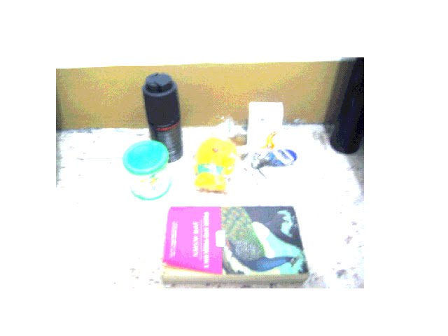
In order to reduce space and send image data without losing a lot of information contain in the original image, the use of PCA in image compression is used. Figure 1 shows the same image to be compressed.

Figure 1: Original Uncompressed Image

We need to slice this image into 10x10 blocks and arrange it into a matrix. Figure 2 shows the stacked sliced blocks.

Figure 2: Chopped Image Blocks

We then perform the principal component analysis and determine the primary eigenvalues and eigenvectors of the image. Figure 3 shows the results of PCA.

Figure 3: Eigenvalue and Correlation results from PCA.

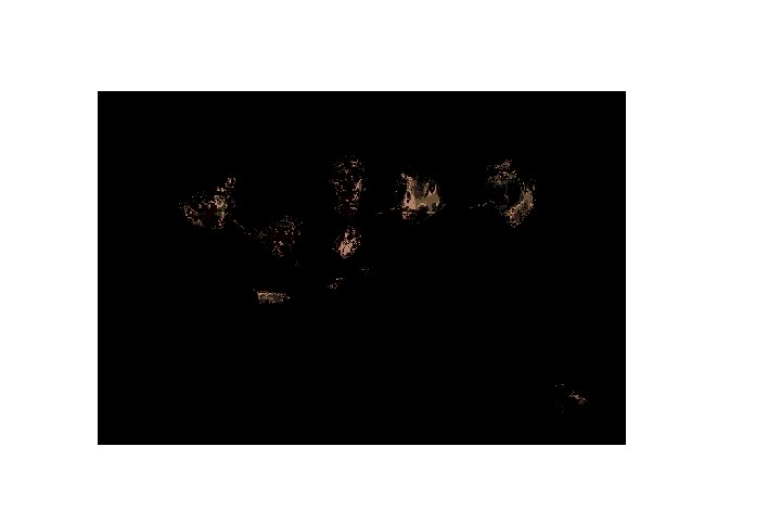
From this information we can compress the image by filtering out eigenvalues and eigenvectors that does not contribute too much on the information on the image. It can be seen that the largest eigenvalue comprises 85% of all the information in the image and in doing so we can reconstruct the image using only this eigenvalue and determine if the image reconstructed still resembles the original image.

Figure 4: 85% confidence reconstructed Image

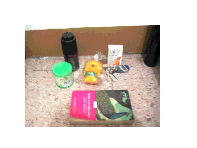
The reconstructed image resembles the original image with 85% confidence and thus we have proven that by reducing the number of eigenvectors used to reconstruct the image we still recovered the image. Figure 5 shows a 90% reconstruction of the image using more eigenvectors.

Figure 5: 90% Accuracy/Confidence Image Reconstruction

References:

[1] M. Soriano, "Activity 14: Image Compression", AP 186, 2010

Self Evaluation: 10

Activity 13: Color Image Segmentation

Results:

Sometimes it is necessary to perform Image processing not on grayscale image but on colored images specially when there is a need to isolated a ROI which is characterized by its color property. Here we investigate two types of algorithms used in colored image segmentation. For the first part we discuss the algorithm for parametric probability distribution. Figure 1 shows the sample image to be used.

Figure 1: Tetris Game Image to be used for Color Segmentation

First, we need to have a basis image wherein that image would be the one which we want to detect. Figure 2 shows some sample patches.

Figure 2: Patches of Tetris blocks to be used in Color Segmentation

We further need to convert these images into rgI format wherein:

r = R/(R+G+B)

g = G/(R+G+B)

I = R+G+B

Figure 3: rgI converted Images

We then determine the mean and standard deviation of pixels values in the red and green layer and use a gaussian function to determine the probability of a pixels belonging to the patch or not.

Figure 4: p(g)p(r) plots for each of the images above.

Using this and applying the probability function for each pixel we can create a mask that when multiplied to the image will result in filtering the unwanted portions.

Figure 5: Segmented Images after applying mask from Parametric algorithm

Another Algorithm uses a non parametric approach wherein we take the 2D histogram of the slice and use it to map out the pixels in the image using histogram back-projection. Using these method and creating another mask to use in the image we try to detect skin on an image show in Figure 6.

Figure 6: Sample image with some SKIN!!

We take a sample slice of a skin and use it to detect other skins. First we need to convert it to rgI again. Figure 7 shows the skin and its rgI image.

Figure 7: Skin(left) rgI of skin(right)

Then we use take the histogram and backproject it to create the mask. Figure 8 shows the histogram and the masked image using 8 bins on the 2d histogram.

Figure 8: 2D histogram of skin patch(8 bins)[top left]; Mask from backprojection[top right], Masked image[bottom]

As we increase the bin size it can be seen that the masked image detects less skin since it could represent more pixels and thus being too specific on the pixels present in the skin patch Figure 9 shows these images.

Figure 9: Masked Images from Histogram(Top to Bottom)[16, 32, 64, 128, 256] Bins.

References:

[1] M. Soriano, "Activity 13:Color Image Segmentation", AP 186, 2010

Self Evaluation: 10

Activity 12: Color Camera Processing

Results:

Images differ depending on the light source it has been captured. Our brain has the capacity to balance an image depending on what it knows to be color white. This process is called white balancing and this algorithm is also used by cameras to correct an image and make it look natural. There are two white balancing algorithms commonly used. First is the white path algorithm wherein you divide the pixel values of the image by the pixel value of the white object. Another is the gray world algorithm wherein you consider the assumption that the world is gray and thus divide the pixel values of the image by the average of all pixel value on the image. Figures below show the process of white balancing images with incorrect white balance settings. All of the images are captured from a flourescent light source and different white balancing settings are used.

Figure 1: Original Image (Cloudy White Balance)[Top], White Patch Algorithm [Middle], Gray World Algorithm [Buttom]

White Patch Algorithm:

Rw = 0.5921569

Gw = 0.6235294

Bw = 0.5333333

Gray World Algorithm:

Rw = 0.3592001

Gw = 0.3325416

Bw = 0.2280096

Figure 2: Original Image (Day Light White Balance)[Top], White Patch Algorithm [Middle], Gray World Algorithm [Buttom]

White Patch Algorithm:

Rw = 0.5058824

Gw = 0.5568627

Bw = 0.5215686

Gray World Algorithm:

Rw = 0.3326466

Gw = 0.3326723

Bw = 0.2590823

Figure 3: Original Image (Fluorescent High White Balance)[Top], White Patch Algorithm [Middle], Gray World Algorithm [Buttom]

White Patch Algorithm:

Rw = 0.5490196

Gw = 0.5333333

Bw = 0.5294118

Gray World Algorithm:

Rw = 0.3809007

Gw = 0.3120621

Bw = 0.2727691

Figure 4: Original Image (Fluorescent White Balance)[Top], White Patch Algorithm [Middle], Gray World Algorithm [Buttom]

White Patch Algorithm:

Rw = 0.5254902

Gw = 0.5647059

Bw = 0.6117647

Gray World Algorithm:

Rw = 0.3553569

Gw = 0.342048

Bw = 0.3251807

Figure 5: Original Image (Tungsten White Balance)[Top], White Patch Algorithm [Middle], Gray World Algorithm [Buttom]

White Patch Algorithm:

Rw = 0.4

Gw = 0.5568627

Bw = 0.7607843

Gray World Algorithm:

Rw = 0.2765657

Gw = 0.3423595

Bw = 0.4473613

In determining which of the two algorithms is better, we take another picture with object with almost the same color. We apply the algorithms and Figure 6 shows the results.

Figure 5: Test Image (Tungsten White Balance)[Top], White Patch Algorithm [Middle], Gray World Algorithm [Buttom]

The white patch algorithms shows a better image quality compared to the gray world algorithm. That is to say even though the white patch algorithm requires the pinpointing of the object that is supposed to be white, the image reconstructed is better. The gray world algorithm on the other hand works best if the image being processed has many colors represented. If this is the case the balancing value represents the average of almost all the colors and thus give a better reconstruction:

References:

[1] M.Soriano,"Activity 12: Color Camera Processing", AP 186, 2010

Self Evaluation: 10