Activity 3:

Results

Image Types

Binary Image

A Binary Image is an image with either black or white pixels.

Figure 1: Sample Binary Image

File Characteristics:

Size: 140 x 200 pixels

File size: 2660 bytes

Format: PNG

Depth: 8

Storage Type: Indexed

Number of Colors: 2

Resolution unit: centimeter

X resolution: 72.00

Y resolution: 72.00

Map = [[0. 0. 0.],[1. 1. 1.]]

Gray-scale Images:

These are images with black and white colors in it. Compared to binary images with only two possible values for each pixel, a grayscale image pixel value can range from 0(black) or 255(white).

Figure 2: Sample Grayscale image

File characteristics:

Size: 300 x 450 pixels

File Size: 77088 bytes

Format: JPEG

Depth: 8

Storage Type: Truecolor

Number of colors: 0

Resolution unit: inch

X resolution: 180.00

Y resolution: 180.00

True Color Images

Images with intesity values of red green and blue.

Figure 3: True color Image sample

File Characteristics:

Size: 480 x 640 pixels

File Size: 32129 bytes

Format: JPEG

Depth: 8

Storage Type: True color

Number of Colors: 0

Resolution unit: inch

X resolution: 96.00

Y resolution: 96.00

Indexed Images

Images with colors referenced to a colormap index.

Figure 4: Sample Indexed Image

File Characteristics

Size: 462 x 453 pixels

FileSize: 12855

Format: GIF

Depth: 8

StorageType: indexed

NumberOfColors: 16

ResolutionUnit: centimeter

XResolution: 72.00

YResolution: 72.00

Advanced Imaging Techniques and Devices:

High Dynamic Range Images

HDRI

Hyperspectral Images

HI

3D Images

3DI

Images can be converted using numerical manipulation and thresholding of the pixel values. Using the image show in Figure 3 we can convert the image into a binary or grayscale image.

Figure 5: Truecolor image converted to binary image format.

Figure 6: Truecolor image converted to grayscale image.

We could further improve the quality of the binary image by taking the histogram of the image and determining the threshold value used in the conversion. Figure 7 shows the histogram of Figure 6.

Figure 7: Histogram of pixel values for the image in Figure 6

We could select the threshold value to 0.4 to remove some of the excess white colors in the figure. In doing this improvement in the image quality as seen in Figure 8.

Figure 8: Improve Binary image of Figure 4.

We can clearly see the in comparison to the initial conversion to the binary image this image has increase in quality by the improvement of the clarity of the title of the book introduction to quantum mechanics wherein in the previous conversion the quantum part is not well defined.

References:

[1] Soriano, M, "Activity 3: Image Types and Formats 2010", AP 186

Acknowledgements: Thank you ma'am jing for your assistance in saving the graphs.

Self evalutaion: 10

Justification: Images required are produced and the the improvement in the thresholding can be seen in the results.

Activity 2: Scilab Basics 2010

Activity 2: Report

Figure 1: Circular Aperture 100x100 pixels

Figure 2: Circular Aperture 200x200 pixels

Figures 1 and 2 show the increase in smoothness as the number of pixels increases. This can directly be explained through the increase in the number of pixels available in representing a portion of an image.

Code: Circular Aperture

nx = 100; ny = 100; //defines the number of elements along x //and y

x = linspace(-1, 1, nx); //defines the range

y = linspace(-1, 1, ny);

[X, Y] = ndgrid(x, y); //creates two 2-D arrays of x and y //coordinates

r = sqrt(X.^2 + Y.^2); //note element-per-element squaring of X //and Y

A = zeros(nx, ny); //creates a 2-D array of zeros with size

//nx X ny

A(find(r <> //locates the indices on the array where //the condition is satisfied and replaces //the value of the element with the same //index on A.

imwrite(A, ‘circularaperture.bmp’) //saves the an image of the //variable A with filename //‘circularaperture.bmp’

imshow(A, []);

Figure 3: Centered Square Aperture

Code: Centered Square Aperture

nx = 500; ny = 500;

x = linspace(-1, 1, nx);

y = linspace(-1, 1, ny);

[X, Y] = ndgrid(x, y);

A = zeros(nx, ny);

A(find(abs(X) <> //Condition for

A(find(abs(Y) <> //square aperture

imwrite(A, ‘centeredsquareaperture.bmp’)

imshow(A, []);

Figure 4: Sinusoid along the X direction

Code: Sinusoid along the X direction

nx = 500; ny = 500;

x = linspace(-1, 1, nx);

y = linspace(-1, 1, ny);

[X, Y] = ndgrid(x, y);

A = (sin(X) + 1.0) / 2.0 //creates a sine wave in the x direction and adjusts //the minimum to 0.0 and maximum to 1.0

imwrite(A, ‘sinusoidinx.bmp’)

imshow(A, []);

Figure 5: Grating along the x direction

Code: Grating along the x direction

nx = 500; ny = 500;

x = linspace(-1, 1, nx);

y = linspace(-1, 1, ny);

[X, Y] = ndgrid(x, y);

A = zeros(nx, ny);

A(find(abs(X)<0.1))> //generates grating strips

A(find((abs(X)<0.5)&(abs(x)>0.3))) = 1; //of width = 0.2 along

A(find((abs(X)<0.9)&(abs(x)>0.7))) = 1; //the x direction

imwrite(A, ‘grating.bmp’)

imshow(A, []);

Figure 6: Annulus

Code: Annulus

nx = 100; ny = 100;

x = linspace(-1, 1, nx);

y = linspace(-1, 1, ny);

[X, Y] = ndgrid(x, y);

r = sqrt(X.^2 + Y.^2);

A = zeros(nx, ny);

A(find((r <>0.4))) = 1; //condition for annular ring of thickness //with outer radius of 0.7 and inner radius //of 0.4

imwrite(A, ‘annulus.bmp’)

imshow(A, []);

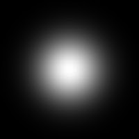
Figure 7: Circular Aperture with Graded Gaussian Transparency

Code: Circular Aperture with Graded Gaussian Transparency

nx = 100; ny = 100;

x = linspace(-1, 1, nx);

y = linspace(-1, 1, ny);

[X, Y] = ndgrid(x, y);

r = sqrt(X.^2 + Y.^2);

A = exp(-5*(r.^2)) //equation for a 2D-Gaussian centered at the origin

imwrite(A, ‘gradedgaussian.bmp’)

imshow(A, []);

Figure 8: Product of two sinusoids in x and y (Egg Container)

Code: Product of two sinusoids in x and y

nx = 100; ny = 100;

x = linspace(-1, 1, nx);

y = linspace(-1, 1, ny);

[X, Y] = ndgrid(x, y);

A = sin(20*X).*sin(20*Y) //Equation for Egg container where element-wise //multiplication is performed

imwrite(A, ‘circularwave.bmp’)

imshow(A, []);

Figure 9: Circular Wave with constant amplitude

Code: Circular Wave with constant amplitude

nx = 100; ny = 100;

x = linspace(-1, 1, nx);

y = linspace(-1, 1, ny);

[X, Y] = ndgrid(x, y);

r = sqrt(X.^2 + Y.^2);

A = (sin(20*r) + 1.0) / 2.0 //Spherical wave with min value = 0.0

//and max value = 1.0

imwrite(A, ‘circularwave.bmp’)

imshow(A, []);

Figure 10: Shifted Circular Gaussian Aperture

Code: Shifted Circular Gaussian Aperture

nx = 100; ny = 100;

x = linspace(-1, 1, nx);

y = linspace(-1, 1, ny);

[X, Y] = ndgrid(x, y);

r = sqrt((X-0.2).^2 + (Y-0.5).^2); //r values are shifted to X = 0.2 and Y = 0.5

A = exp(-5*(r.^2))

imwrite(A, ‘shiftedgaussian.bmp’)

imshow(A, []);

References:

[1] Soriano, M., "Activity 2: Scilab Basics 2010", AP 186

Self Evaluation: 10

Justification: Images produced are of good quality and all required results are presented completely.

Self Evaluation: Activity 1

Rating: 10

Justification: The data points coincide perfectly with the original graph. This means that the approach for the ratio and proportion is correct. The labels of the data points are also included just as what was in the graph.

References: Journal for Experiemtal Zoology.

Digital Scanning

Digital Scanning

RESULTS

Figure 1. Scanned Hand draw graph.

Data from the hand drawn graph can be extracted by the use information taken from the positions of the pixels where data points are located. By the use of ratio and proportion, one can reconstruct the hand drawn graph and retrieve the values of the data points. For a scanned image, a pixel has an X and Y position, however, the positions of its (0,0) is not at the bottom left edge but at the upper left edge. Due to this the computation for the Y value is not just a simple ratio and proportion but we must include the difference in the orientation of the coordinate systems.

After taking the pixel positions of each data point, we must also get the positions of the axis ticks and the position of the graph edge. For this graph it is the value (10 degrees Celsius, 25 seconds). It is important to take the edge of the graphs since it is the graph values that you are scaling and not the image itself. Extra spaces in the graph if not considered may include errors in the computation of the values. After taking the positions of the tick marks in the axes and knowing the tick length from the original graph, one can calculate the constant of proportionality for X, Y by subtracting the pixel positions of consecutive tick marks. Divide the tick length by this value and you will obtain the proportionality constant (physical value / pixel).

In calculating the values of the data points from pixel positions. For the x position, we must first subtract the x position of the graph edge to the x pixel position of the data point,then multiply the result to the x proportionality constant, then add x value(physical value) of the graph edge. For the y position, we must first subtract the y pixel position of the data point to the y position of the graph edge, then we can proceed with multiplying the constant and the addition of the y initial value.

X proportionality constant: 0.043796

Y proportionality constant: 0.088496

X graph edge position: 259

Y graph edge position: 1073

X initial value: 10

Y initial value: 25

Equations:

Xval = ((Xpos - Xgraphedge) * Xconst) + Xin

Yval = ((Ygraphedge - Ypos) * Yconst) + Yin

Figure 2: Reconstructed graph from pixel information

The reconstructed graph shows that hand drawn graphs can be reconstructed using pixel position values.

Figure 3: Overlaying of the Hand drawn graph and the reconstructed graph

The overlaying of the two graphs shows that the pixel value information can be used to retrieve information about the data point on the graph by simple ratio and proportion. The graph shows that all computed data points coincide with those of the hand drawn graph. However the trend-line of the graphs did not coincide since both graphs used different fitting techniques. The reconstructed graph used error minimization techniques to form the fit, while the hand drawn graph used a French curve to make the line smoother compared to connect-the-dots technique.