Activity 2: Scilab Basics 2010

Activity 2: Report

Figure 1: Circular Aperture 100x100 pixels

Figure 2: Circular Aperture 200x200 pixels

Figures 1 and 2 show the increase in smoothness as the number of pixels increases. This can directly be explained through the increase in the number of pixels available in representing a portion of an image.

Code: Circular Aperture

nx = 100; ny = 100; //defines the number of elements along x //and y

x = linspace(-1, 1, nx); //defines the range

y = linspace(-1, 1, ny);

[X, Y] = ndgrid(x, y); //creates two 2-D arrays of x and y //coordinates

r = sqrt(X.^2 + Y.^2); //note element-per-element squaring of X //and Y

A = zeros(nx, ny); //creates a 2-D array of zeros with size

//nx X ny

A(find(r <> //locates the indices on the array where //the condition is satisfied and replaces //the value of the element with the same //index on A.

imwrite(A, ‘circularaperture.bmp’) //saves the an image of the //variable A with filename //‘circularaperture.bmp’

imshow(A, []);

Figure 3: Centered Square Aperture

Code: Centered Square Aperture

nx = 500; ny = 500;

x = linspace(-1, 1, nx);

y = linspace(-1, 1, ny);

[X, Y] = ndgrid(x, y);

A = zeros(nx, ny);

A(find(abs(X) <> //Condition for

A(find(abs(Y) <> //square aperture

imwrite(A, ‘centeredsquareaperture.bmp’)

imshow(A, []);

Figure 4: Sinusoid along the X direction

Code: Sinusoid along the X direction

nx = 500; ny = 500;

x = linspace(-1, 1, nx);

y = linspace(-1, 1, ny);

[X, Y] = ndgrid(x, y);

A = (sin(X) + 1.0) / 2.0 //creates a sine wave in the x direction and adjusts //the minimum to 0.0 and maximum to 1.0

imwrite(A, ‘sinusoidinx.bmp’)

imshow(A, []);

Figure 5: Grating along the x direction

Code: Grating along the x direction

nx = 500; ny = 500;

x = linspace(-1, 1, nx);

y = linspace(-1, 1, ny);

[X, Y] = ndgrid(x, y);

A = zeros(nx, ny);

A(find(abs(X)<0.1))> //generates grating strips

A(find((abs(X)<0.5)&(abs(x)>0.3))) = 1; //of width = 0.2 along

A(find((abs(X)<0.9)&(abs(x)>0.7))) = 1; //the x direction

imwrite(A, ‘grating.bmp’)

imshow(A, []);

Figure 6: Annulus

Code: Annulus

nx = 100; ny = 100;

x = linspace(-1, 1, nx);

y = linspace(-1, 1, ny);

[X, Y] = ndgrid(x, y);

r = sqrt(X.^2 + Y.^2);

A = zeros(nx, ny);

A(find((r <>0.4))) = 1; //condition for annular ring of thickness //with outer radius of 0.7 and inner radius //of 0.4

imwrite(A, ‘annulus.bmp’)

imshow(A, []);

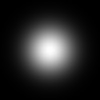
Figure 7: Circular Aperture with Graded Gaussian Transparency

Code: Circular Aperture with Graded Gaussian Transparency

nx = 100; ny = 100;

x = linspace(-1, 1, nx);

y = linspace(-1, 1, ny);

[X, Y] = ndgrid(x, y);

r = sqrt(X.^2 + Y.^2);

A = exp(-5*(r.^2)) //equation for a 2D-Gaussian centered at the origin

imwrite(A, ‘gradedgaussian.bmp’)

imshow(A, []);

Figure 8: Product of two sinusoids in x and y (Egg Container)

Code: Product of two sinusoids in x and y

nx = 100; ny = 100;

x = linspace(-1, 1, nx);

y = linspace(-1, 1, ny);

[X, Y] = ndgrid(x, y);

A = sin(20*X).*sin(20*Y) //Equation for Egg container where element-wise //multiplication is performed

imwrite(A, ‘circularwave.bmp’)

imshow(A, []);

Figure 9: Circular Wave with constant amplitude

Code: Circular Wave with constant amplitude

nx = 100; ny = 100;

x = linspace(-1, 1, nx);

y = linspace(-1, 1, ny);

[X, Y] = ndgrid(x, y);

r = sqrt(X.^2 + Y.^2);

A = (sin(20*r) + 1.0) / 2.0 //Spherical wave with min value = 0.0

//and max value = 1.0

imwrite(A, ‘circularwave.bmp’)

imshow(A, []);

Figure 10: Shifted Circular Gaussian Aperture

Code: Shifted Circular Gaussian Aperture

nx = 100; ny = 100;

x = linspace(-1, 1, nx);

y = linspace(-1, 1, ny);

[X, Y] = ndgrid(x, y);

r = sqrt((X-0.2).^2 + (Y-0.5).^2); //r values are shifted to X = 0.2 and Y = 0.5

A = exp(-5*(r.^2))

imwrite(A, ‘shiftedgaussian.bmp’)

imshow(A, []);

References:

[1] Soriano, M., "Activity 2: Scilab Basics 2010", AP 186

Self Evaluation: 10

Justification: Images produced are of good quality and all required results are presented completely.